Using Lustre¶

File systems on LUMI¶

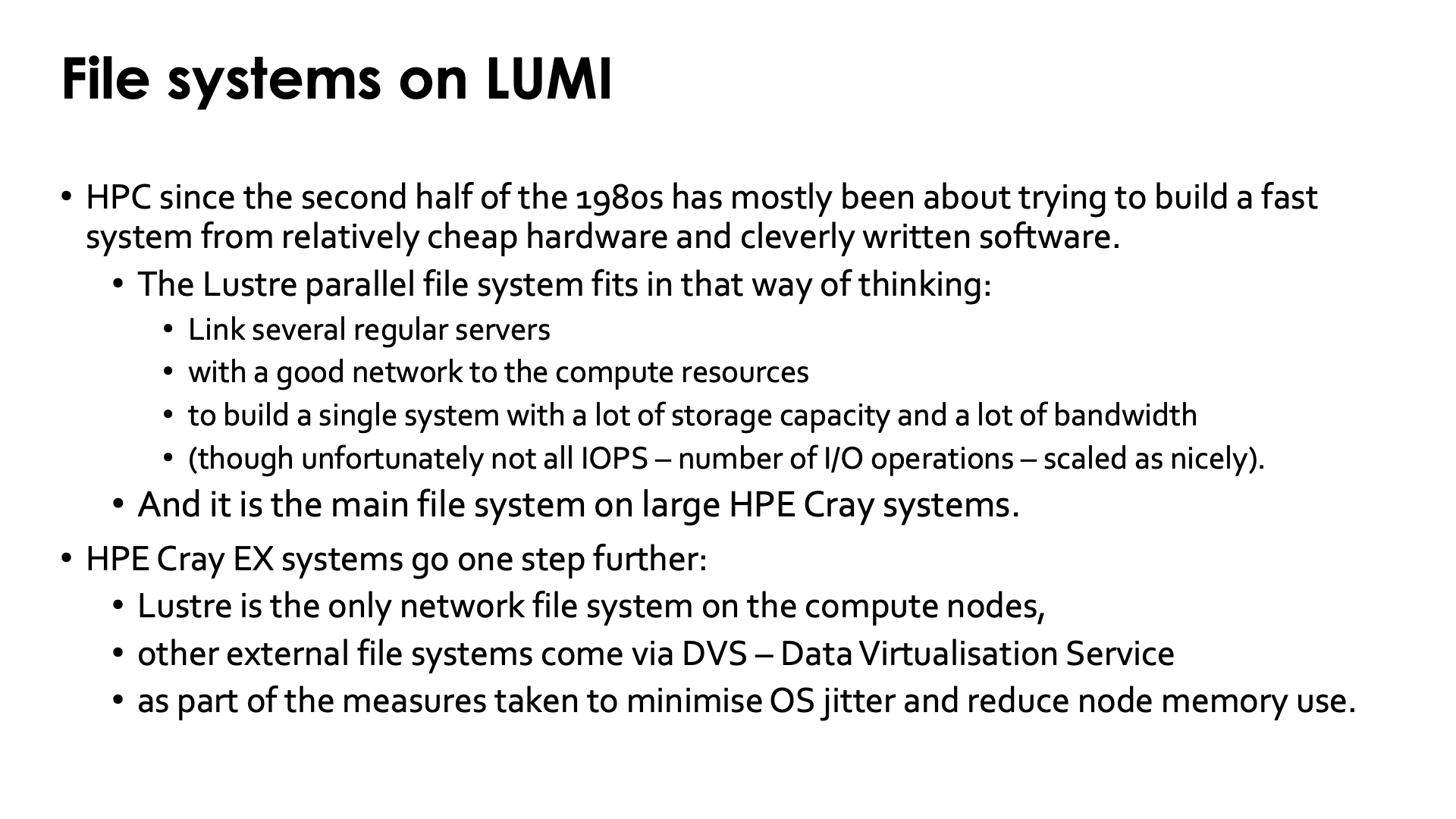
Supercomputing since the second half of the 1980s has almost always been about trying to build a very fast system from relatively cheap volume components or technologies (as low as you can go without loosing too much reliability) and very cleverly written software both at the system level (to make the system look like a true single system as much as possible) and at the application level (to deal with the restrictions that inevitably come with such a setup).

The Lustre parallel file system that we use on LUMI (and that is its main file system serving user files) fits in that way of thinking. A large file system is built by linking many fairly regular file servers through a fast network to the compute resources to build a single system with a lot of storage capacity and a lot of bandwidth. It has its restrictions also though: not all types of IOPs (number of I/O operations per second) scale as well or as easily as bandwidth and capacity so this comes with usage restrictions on large clusters that may a lot more severe than you are used to from small systems. And yes, it is completely normal that some file operations are slower than on the SSD of a good PC.

HPE Cray EX systems go even one step further. Lustre is the only network file system directly served to the compute nodes. Other network file system come via a piece of software called Data Virtualisation Service (abbreviated DVS) that basically forwards I/O requests to servers in the management section of the cluster where the actual file system runs. This is part of the measures that Cray takes in Cray Operating System to minimise OS jitter on the compute nodes to improve scalability of applications, and to reduce the memory footprint of the OS on the compute nodes.

Lustre building blocks¶

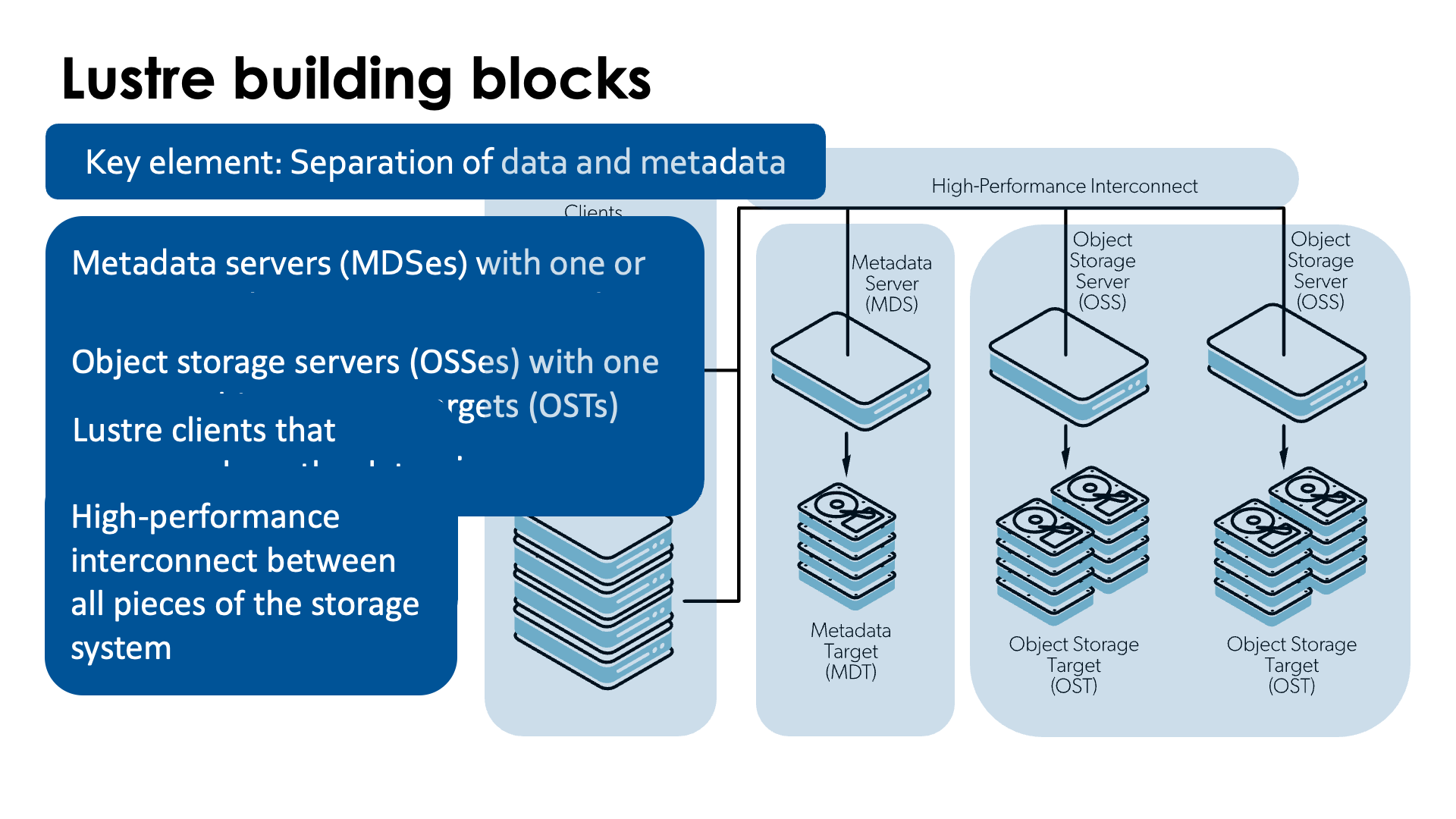
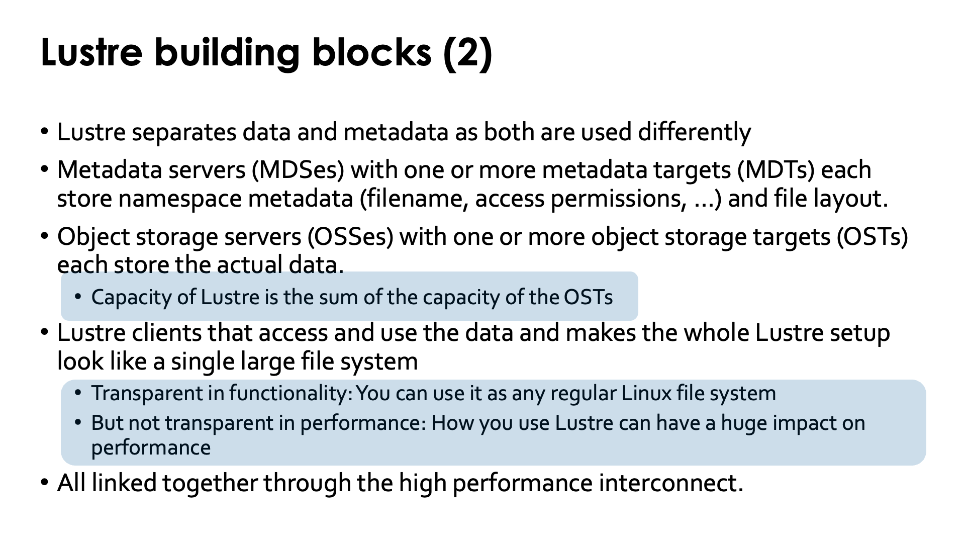
A key element of Lustre - but also of other parallel file systems for large parallel computers such as BeeGFS, Spectrum Scale (formerly GPFS) or PanFS - is the separation of metadata and the actual file data, as the way both are accessed and used is very different.

A Lustre system consists of the following blocks:

Metadata servers (MDSes) with one or more metadata targets (MDTs) each store namespace metadata such as filenames, directories and access permissions, and the file layout.

Each MDT is a filesystem, usually with some level of RAID or similar technologies for increased reliability. Usually there is also more than one MDS and they are put in a high availability setup for increased availability (and this is the case in LUMI).

Metadata is accessed in small bits and it does not need much capacity. However, metadata accesses are hard to parallelise so it makes sense to go for the fastest storage possible even if that storage is very expensive per terabyte. On LUMI all metadata servers use SSDs.
Object storage servers (OSSes) with one or more object storage targets (OSTs) each store the actual data. Data from a single file can be distributed across multiple OSTs and even multiple OSSes. As we shall see, this is also the key to getting very high bandwidth access to the data.

Each OST is a filesystem, again usually with some level of RAID or similar technologies to survive disk failures. One OSS typically has between 1 and 8 OSTs, and in a big setup a high availability setup will be used again (as is the case in LUMI).

The total capacity of a Lustre file system is the sum of the capacity of all OSTs in the Lustre file system. Lustre file systems are often many petabytes large.

Now you may think differently based upon prices that you see in the PC market for hard drives and SSDs, but SSDs of data centre quality are still up to 10 times as expensive as hard drives of data centre quality. Building a file system of several tens of petabytes out of SSDs is still extremely expensive and rarely done, certainly in an environment with a high write pressure on the file system as that requires the highest quality SSDs. Hence it is not uncommon that supercomputers will use mostly hard drives for their large storage systems.

On LUMI there is roughly 80 PB spread across 4 large hard disk based Lustre file systems, and 8.5 PB in an SSD-based Lustre file system. However, all MDSes use SSD storage.
Lustre clients access and use the data. They make the whole Lustre file system look like a single file system.

Lustre is transparent in functionality. You can use a Lustre file system just as any other regular file system, with all your regular applications. However, it is not transparent when it comes to performance: How you use Lustre can have a huge impact on performance. Lustre is optimised very much for high bandwidth access to large chunks of data at a time from multiple nodes in the application simultaneously, and is not very good at handling access to a large pool of small files instead.

So you have to store your data (but also your applications as the are a kind of data also) in an appropriate way, in fewer but larger files instead of more smaller files. Some centres with large supercomputers will advise you to containerise software for optimal performance. On LUMI we do advise Python users or users who install software through Conda to do so.
All these components are linked together through a high performance interconnect. On HPE Cray EX systems - but on more an more other systems also - there is no separate network anymore for storage access and the same high performance interconnect that is also used for internode communication by applications (through, e.g., MPI) is used for that purpose.
There is also a management server which is not mentioned on the slides, but that component is not essential to understand the behaviour of Lustre for the purpose of this lecture.

Links

Striping: Large files are spread across OSTs¶

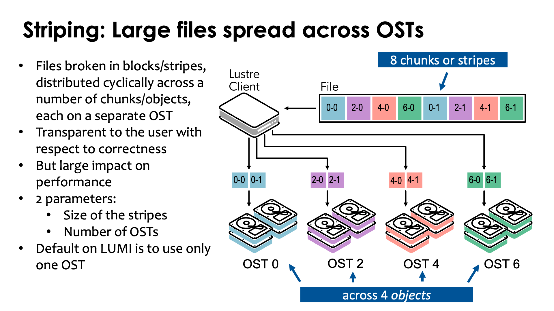
On Lustre, large files are typically broken into blocks called stripes or chunks that are then cyclically spread across a number of chunk files called objects in LUSTRE, each on a separate OST. In the figure in the slide above, the file is spread across the OSTs 0, 2, 4 and 6.

This process is completely transparent to the user with respect to correctness. The Lustre client takes care of the process and presents a traditional file to the application program. It is however not transparent with respect to performance. The performance of reading and writing a file depends a lot on how the file is spread across the OSTs of a file system.

Basically, there are two parameters that have to be chosen: The size of the stripes (all stripes have the same size in this example, except for the last one which may be smaller) and the number of OSTs that should be used for a file. Lustre itself takes care of choosing the OSTs in general.

There are variants of Lustre where one has multiple layouts per file which can come in handy if one doesn't know the size of the file in advance. The first part of the file will then typically be written with fewer OSTs and/or smaller chunks, but this is outside the scope of this course. The feature is known as Progressive File Layout.

The stripe size and number of OSTs used can be chosen on a file-by-file basis. The default on LUMI is to use only one OST for a file. This is done because that is the most reasonable choice for the many small files that many unsuspecting users have, and as we shall see, it is sometimes even the best choice for users working with large files. But it is not always the best choice. And unfortunately there is no single set of parameters that is good for all users.

Objects

The term "object" nowadays has different meanings, even in the storage world. The Object Storage Servers in Lustre should not be confused with the object storage used in cloud solutions such as Amazon Web Services (AWS) with the S3 storage service or the LUMI-O object storage. In fact, the Object Storage Servers use a regular file system such as ZFS or ldiskfs to store the "objects".

Accessing a file¶

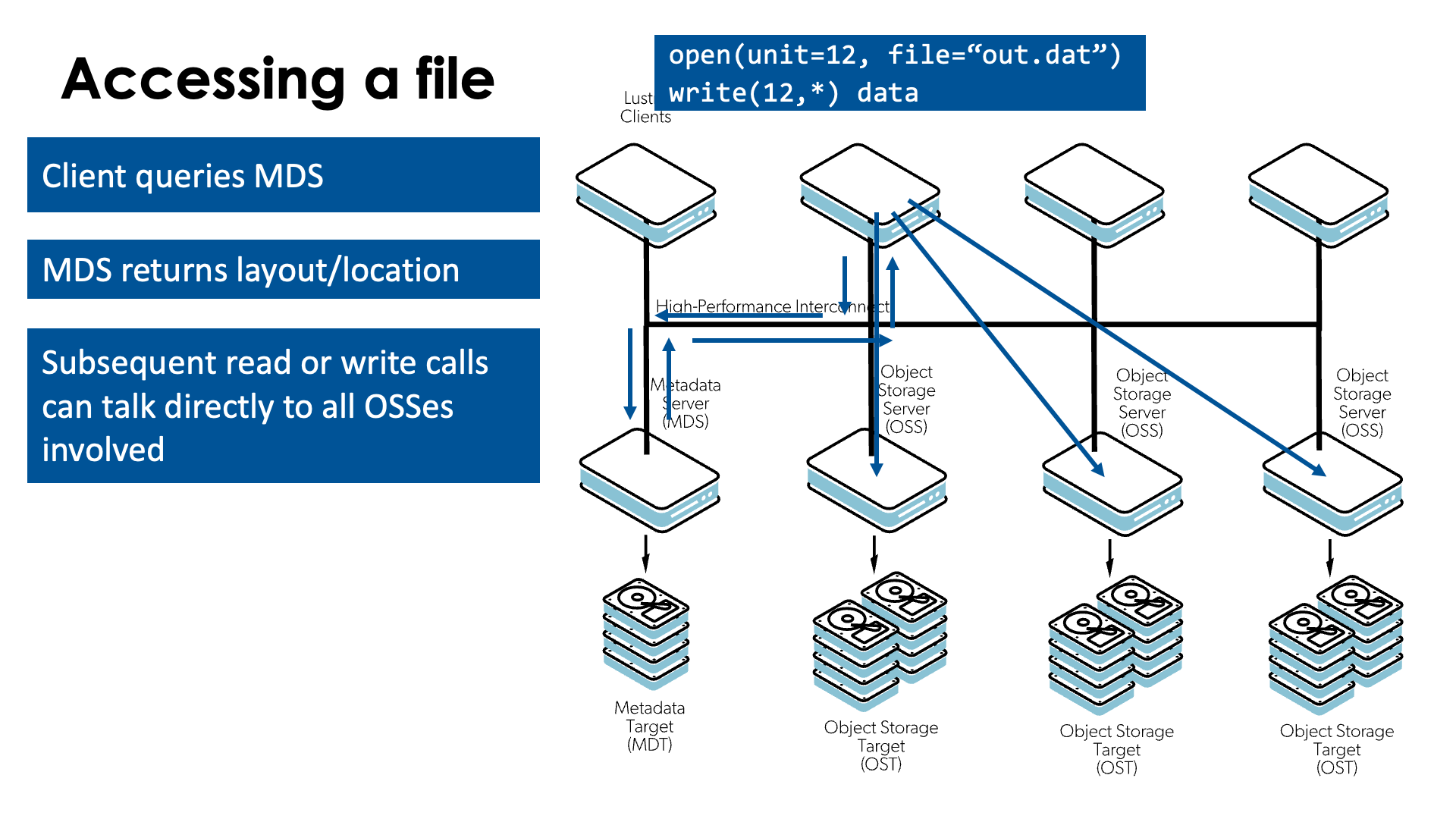
Let's now study how Lustre will access a file for reading or writing. Let's assume that the second client in the above picture wants to write something to the file.

The first step is opening the file.

For that, the Lustre client has to talk to the metadata server (MDS) and query some information about the file.

The MDS in turn will return information about the file, including the layout of the file: chunksize and the OSSes/OSTs that keep the chunks of the file.
From that point on, the client doesn't need to talk to the MDS anymore and can talk directly to the OSSes to write data to the OSTs or read data from the OSTs.

Parallelism is key!¶

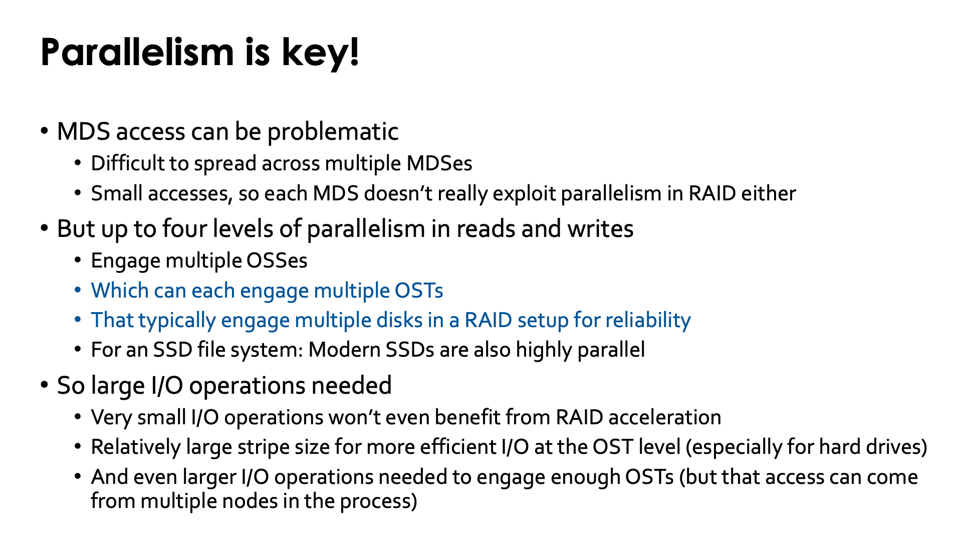
The metadata servers can be the bottleneck in a Lustre setup. It is not easy to spread metadata across multiple MDSes efficiently. Moreover, the amount of metadata for any given file is small, so any metadata operation will translate into small disk accesses on the MDTs and hence not fully exploit the speed that some RAID setups can give you.

However, when reading and writing data, there are up to four levels of parallelism:

The read and write operations can engage multiple OSSes.
Since a single modern OSS can handle more bandwidth than a some OSTs can deliver, OSSes may have multiple OSTs.

How many OSTs are engaged is something that a user has control over.
An OST will contain many disks or SSDs, typically with some kind of RAID, but hence each read or write operation to an OST can engage multiple disks.

An OST will only be used optimally when doing large enough file accesses. But the file system client may help you here with caching.
Internally, SSDs are also parallel devices. The high bandwidth of modern high-end SSDs is the result of engaging multiple channels to the actual storage "chips" internally.

So to fully benefit from a Lustre file system, it is best to work with relatively few files (to not overload the MDS) but very large disk accesses. Very small I/O operations wouldn't even benefit from the RAID acceleration, and this is especially true for very small files as they cannot even benefit from caching provided by the file system client (otherwise a file system client may read in more data than requested, as file access is often sequential anyway so it would be prepared for the next access). To make efficient use of the OSTs it is important to have a relatively large chunk size and relatively large I/O operations, even more so for hard disk based file systems as if the OST file system manages to organise the data well on disk, it is a good way to reduce the impact on effective bandwidth of the inherent latency of disk access. And to engage multiple OSTs simultaneously (and thus reach a bandwidth which is much higher than a single OST can provide), even larger disk accesses will be needed so that multiple chunks are read or written simultaneously. Usually you will have to do the I/O in a distributed memory application from multiple nodes simultaneously as otherwise the bandwidth to the interconnect and processing capacity of the client software of a single node might become the limiting factor.

Not all codes are using Lustre optimally though, even with the best care of their users.

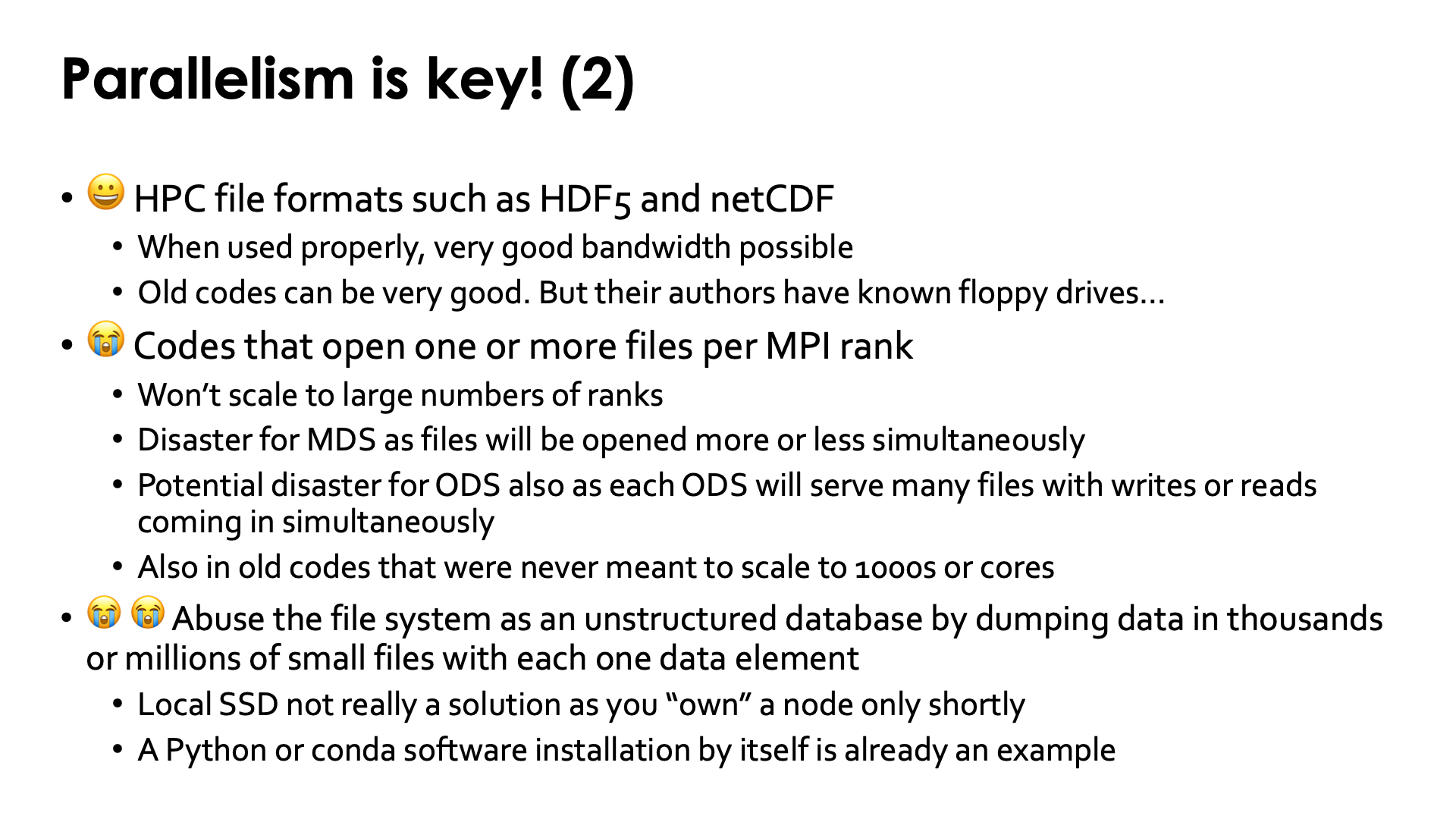
Some codes use files in scientific data formats like HDF5 and netCDF, and when written properly they can have very scalable performance.

A good code will write data to large files, from multiple nodes simultaneously, but will avoid doing I/O from too many ranks simultaneously to avoid bombarding the OSSes/OSTs with I/O requests. But that is a topic for a more advanced course...

One user has reported reading data from the hard disk based parallel file systems at about 25% of the maximal bandwidth, which is very good given that other users where also using that file system at the same time and not always in an optimal way.

Surprisingly many of these codes may be rather old. But their authors grew up with noisy floppy drives (do you still know what that is) and slow hard drives so learned how to program efficiently.
But some codes open one or more files per MPI rank. Those codes may have difficulties scaling to a large number of ranks, as they will put a heavy burden on the MDS when those files are created, but also may bombard each OSS/OST with too many I/O requests.

Some of these codes are rather old also, but were never designed to scale to thousands of MPI ranks. However, nowadays some users are trying to solve such big problems that the computations do scale reasonably well. But the I/O of those codes becomes a problem...
But some users simply abuse the file system as an unstructured database and simply drop their data as tens of thousands or even millions of small files with each one data element, rather than structuring that data in suitable file formats. This is especially common in science fields that became popular relatively recently - bio-informatics and AI - as those users typically started their work on modern PCs with fast SSDs.

The problem there is that metadata access and small I/O operations don't scale well to large systems. Even copying such a data set to a local SSD would be a problem should a compute node have a local SSD, but local SSDs suitable for supercomputers are also very expensive as they have to deal with lots of write operations. Your gene data or training data set may be relatively static, but on a supercomputer you cannot keep the same node for weeks so you'd need to rewrite your data to local disks very often. And there are shared file systems with better small file performance than Lustre, but those that scale to the size of even a fraction of Lustre, are also very expensive. And remember that supercomputing works exactly the opposite way: Try to reduce costs by using relatively cheap hardware but cleverly written software at all levels (system and application) as at a very large scale, this is ultimately cheaper than investing more in hardware and less in software.

Lustre was originally designed to achieve very high bandwidth to/from a small number of files, and that is in fact a good match for well organised scientific data sets and/or checkpoint data, but was not designed to handle large numbers of small files. Nowadays of course optimisations to deal better with small files are being made, but they may come at a high hardware cost.

How to determine the striping values?¶

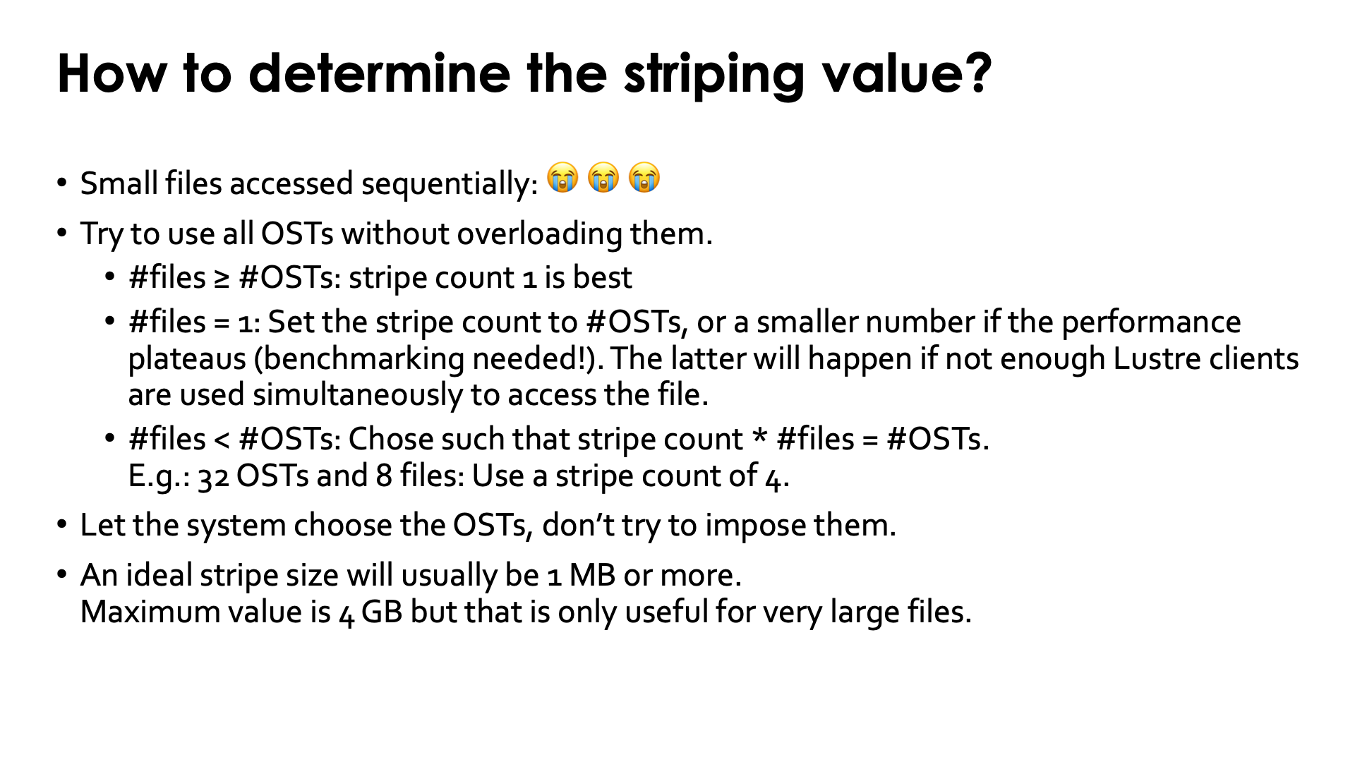
If you only access relatively small files (up to a few hundreds of kilobytes) and access them sequentially, then you are out of luck. There is not much you can do. Engaging multiple OSTs for a single file is not useful at all in this case, and you will also have no parallelism from accessing multiple files that may be stored on different OSTs. The metadata operations may also be rather expensive compared to the cost of reading the file once opened.

As a rule of thumb, if you access a lot of data with a data access pattern that can exploit parallelism, try to use all OSTs of the Lustre file system without unnecessary overloading them:

If the number of files that will be accessed simultaneously is larger than the number of OSTs, it is best to not spread a single file across OSTs and hence use a stripe count of 1.

It will also reduce Lustre contention and OST file locking and as such gain performance for everybody.
At the opposite end, if you access only one very large file and use large or parallel disk accesses, set the stripe count to the number of OSTs (or a smaller number if you notice in benchmarking that the I/O performance plateaus). On a system the size of LUMI with storage as powerful as on LUMI, this will only work if you have more than on I/O client.
When using multiple similar sized files simultaneously but less files than there are OSTs, you should probably chose the stripe count such that the product of the number of files and the stripe count is approximately the number of OSTs. E.g., with 32 OSTs and 8 files, set the stripe count to 4.

It is better not to force the system to use specific OSTs but to let it chose OSTs at random.

The typical stripe size (size of the chunks) to use can be a bit harder to determine. Typically this will be 1MB or more, and it can be up to 4 GB, but that only makes sense for very large files. The ideal stripe size will also depend on the characteristics of the I/O in the file. If the application never writes more than 1 GB of data in a single sequential or parallel I/O operation before continuing with more computations, obviously with a stripe size of 1 GB you'd be engaging only a single OST for each write operation.

Managing the striping parameters¶

The basic Lustre command for regular users to do special operations on Lustre is the lfs command, which has various subcommands.

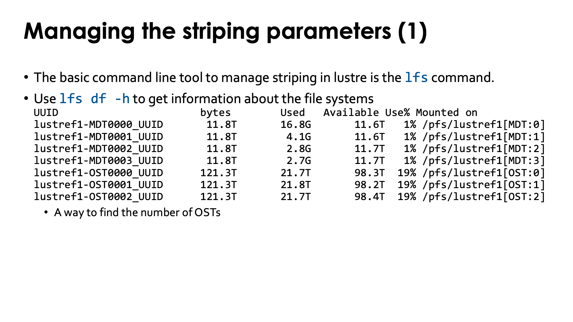
The first interesting subcommand is df which has a similar purpose as the regular Linux df command: Return information about the filesystem. In particular,

lfs df -h

will return information about all available Lustre filesystems. The -h flag tells the command to use "human-readable" number formats: return sizes in gigabytes and terabytes rather than blocks. On LUMI, the output starts with:

$ lfs df -h
UUID                       bytes        Used   Available Use% Mounted on
lustref1-MDT0000_UUID       11.8T       16.8G       11.6T   1% /pfs/lustref1[MDT:0]
lustref1-MDT0001_UUID       11.8T        4.1G       11.6T   1% /pfs/lustref1[MDT:1]
lustref1-MDT0002_UUID       11.8T        2.8G       11.7T   1% /pfs/lustref1[MDT:2]
lustref1-MDT0003_UUID       11.8T        2.7G       11.7T   1% /pfs/lustref1[MDT:3]
lustref1-OST0000_UUID      121.3T       21.5T       98.5T  18% /pfs/lustref1[OST:0]
lustref1-OST0001_UUID      121.3T       21.6T       98.4T  18% /pfs/lustref1[OST:1]
lustref1-OST0002_UUID      121.3T       21.4T       98.6T  18% /pfs/lustref1[OST:2]
lustref1-OST0003_UUID      121.3T       21.4T       98.6T  18% /pfs/lustref1[OST:3]

so the command can also be used to see the number of MDTs and OSTs available in each filesystem, with the capacity.

Striping in Lustre is set at a filesystem level by the sysadmins, but users can adjust the settings at the directory level (which then sets the default for files created in that directory) and file level. Once a file is created, the striping configuration cannot be changed anymore on-the-fly.

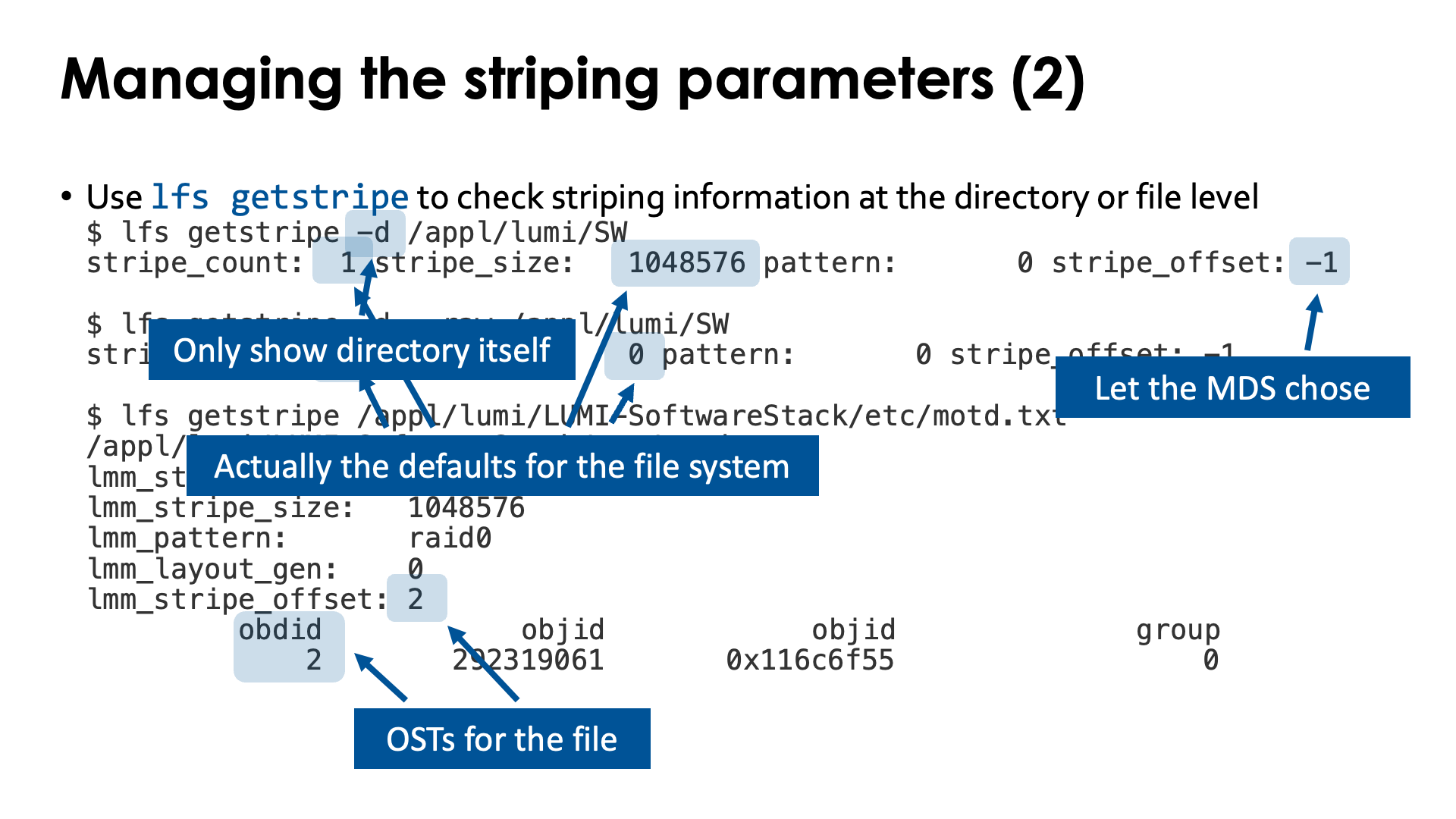
To inspect the striping configuration, one can use the getstripe subcommand of lfs.

Let us first use it at the directory level:

$ lfs getstripe -d /appl/lumi/SW
stripe_count:  1 stripe_size:   1048576 pattern:       0 stripe_offset: -1

$ lfs getstripe -d --raw /appl/lumi/SW
stripe_count:  0 stripe_size:   0 pattern:       0 stripe_offset: -1

The -d flag tells that we only want information about the directory itself and not about everything in that directory. The first lfs getstripe command tells us that files created in this directory will use only a single OST and have a stripe size of 1 MiB. By adding the --raw we actually see the settings that have been made specifically for this directory. The 0 for stripe_count and stripe_size means that the default value is being used, and the stripe_offset of -1 also indicates the default value.

We can also use lfs getstripe for individual files:

$ lfs getstripe /appl/lumi/LUMI-SoftwareStack/etc/motd.txt
/appl/lumi/LUMI-SoftwareStack/etc/motd.txt
lmm_stripe_count:  1
lmm_stripe_size:   1048576
lmm_pattern:       raid0
lmm_layout_gen:    0
lmm_stripe_offset: 10
        obdidx           objid           objid           group
            10        56614379      0x35fddeb                0

Now lfs getstripe does not only return the stripe size and number of OSTs used, but it will also show the OSTs that are actually used (in the column obdidx of the output). The lmm_stripe_offset is also the number of the OST with the first object of the file.

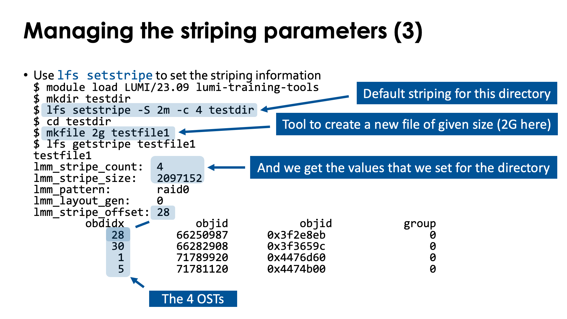
The final subcommand that we will discuss is the setstripe subcommand to set the striping policy for a file or directory.

Let us first look at setting a striping policy at the directory level:

$ module use /appl/local/training/modules/2day-20240502
$ module load lumi-training-tools
$ mkdir testdir
$ lfs setstripe -S 2m -c 4 testdir
$ cd testdir
$ mkfile 2g testfile1
$ lfs getstripe testfile1
testfile1
lmm_stripe_count:  4
lmm_stripe_size:   2097152
lmm_pattern:       raid0
lmm_layout_gen:    0
lmm_stripe_offset: 28
        obdidx           objid           objid           group
            28        66250987      0x3f2e8eb                0
            30        66282908      0x3f3659c                0
             1        71789920      0x4476d60                0
             5        71781120      0x4474b00                0

The lumi-training-tools module provides the mkfile command that we use in this example.

We first create a directory and then set the striping parameters to a stripe size of 2 MiB (the -S flag) and a so-called stripe count, the number of OSTs used for the file, of 4 (the -c flag).

Next we go into the subdirectory and use the mkfile command to generate a file of 2 GiB.

When we now check the file layout of the file that we just created with lfs getstripe, we see that the file now indeed uses 4 OSTs with a stripe size of 2 MiB, and has object on in this case OSTs 28, 30, 1 and 5.

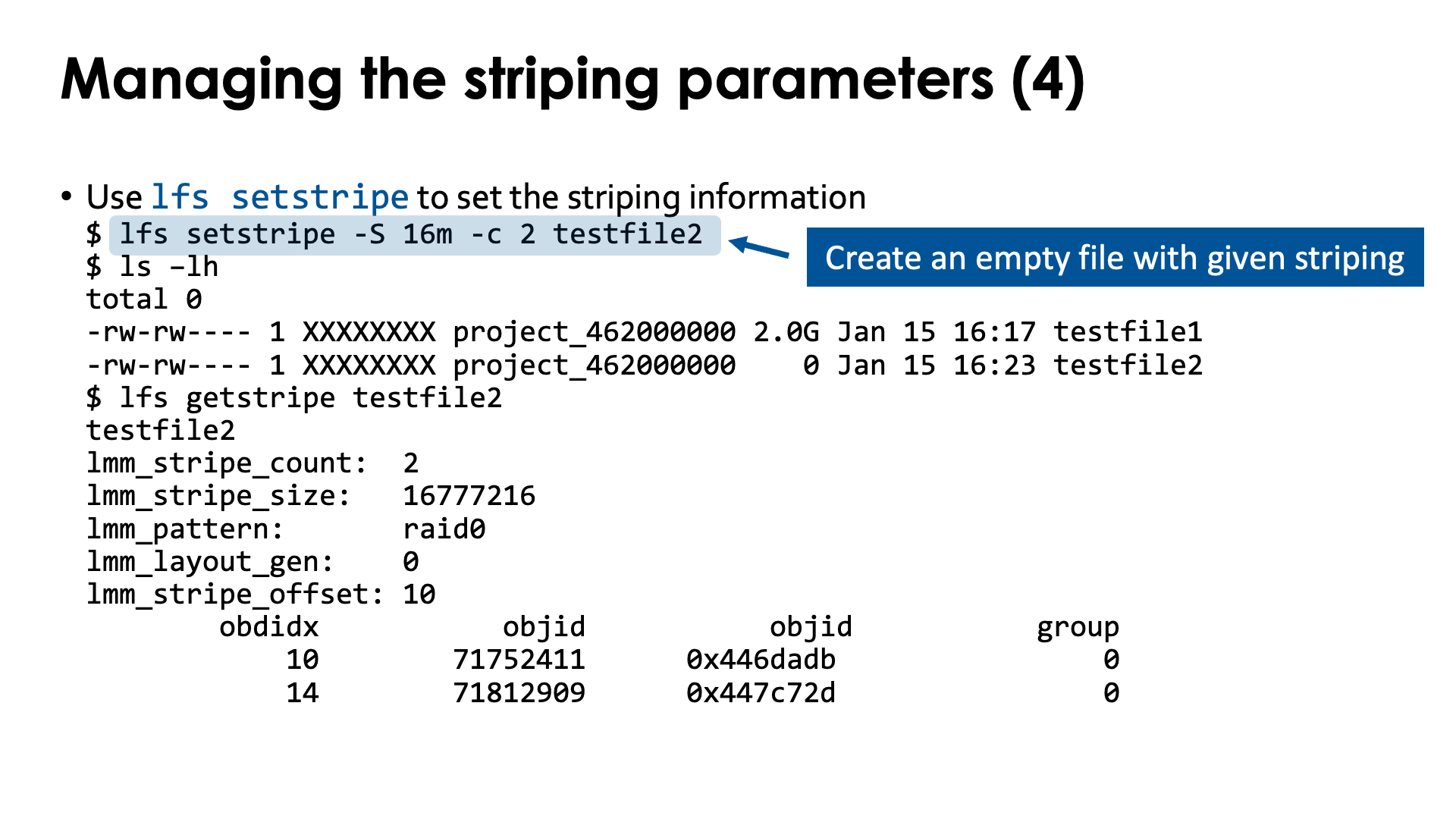
However, we can even control striping at the level of an individual file. The condition is that the layout of the file is set as soon as it is created. We can do this also with lfs setstripe:

$ lfs setstripe -S 16m -c 2 testfile2
$ ls -lh
total 0
-rw-rw---- 1 XXXXXXXX project_462000000 2.0G Jan 15 16:17 testfile1
-rw-rw---- 1 XXXXXXXX project_462000000    0 Jan 15 16:23 testfile2
$ lfs getstripe testfile2
testfile2
lmm_stripe_count:  2
lmm_stripe_size:   16777216
lmm_pattern:       raid0
lmm_layout_gen:    0
lmm_stripe_offset: 10
        obdidx           objid           objid           group
            10        71752411      0x446dadb                0
            14        71812909      0x447c72d                0

In this example, the lfs setstripe command will create an empty file but with the required layout. In this case we have set the stripe size to 16 MiB and use only 2 OSTs, and the lfs getstripe command confirms that information. We can now open the file to write data into it with the regular file operations of the Linux glibc library or your favourite programming language (though of course you need to take into account that the file already exists so you should use routines that do not return an error if the file already exists).

Lustre API

Lustre also offers a C API to directly set file layout properties, etc., from your package. Few scientific packages seem to support it though.

The metadata servers¶

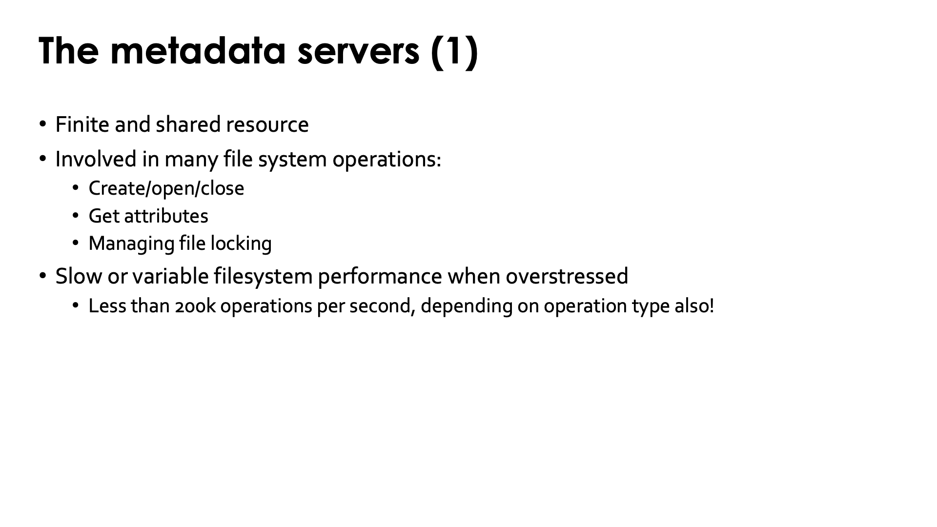
Parallelising metadata access is very difficult. Even large Lustre filesystems have very few metadata servers. They are a finite and shared resource, and overloading the metadata server slows down the file system for all users.

The metadata servers are involved in many operations. The play a role in creating, opening and also closing files. The provide some of the attributes of a file. And they also play a role in file locking.

Yet the metadata servers have a very finite capacity. The Lustre documentation claims that in theory a single metadata server should be capable of up to 200,000 operations per second, depending on the type of request. However, 75,000 operations per second may be more realistic.

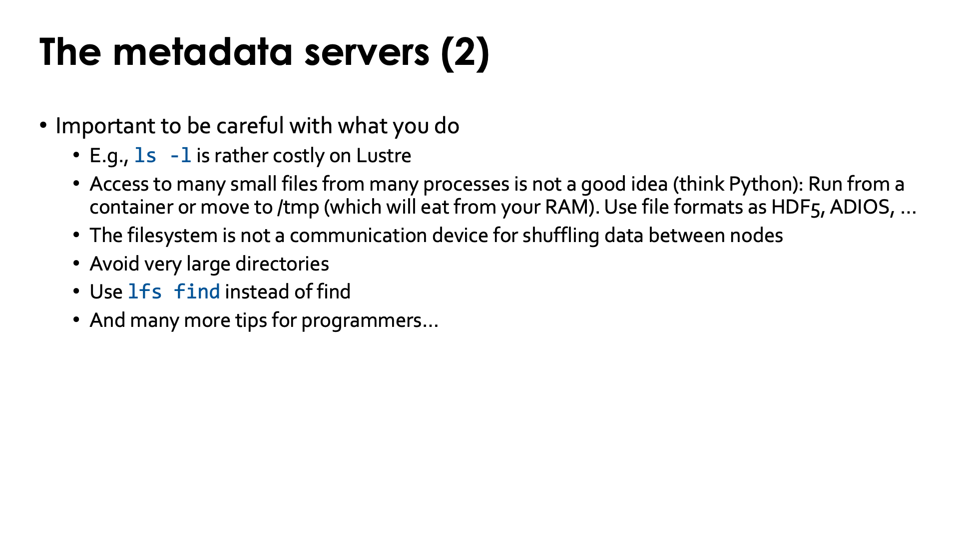
As a user, many operations that you think are harmless from using your PC, are in fact expensive operations on a supercomputer with a large parallel file system and you will find "Lustre best practices" pages on web sites of many large supercomputer centres. Some tips for regular users:

Any command that requests attributes is fairly expensive and should not be used in large directories. This holds even for something as trivial as ls -l. But it is even more so for commands as du that run recursively through attributes of lots of files.
Opening a file is also rather expensive as it involves a metadata server and one or more object servers. It is not a good idea to frequently open and close the same file while processing data.
Therefore access to many small files from many processes is not a good idea. One example of this is using Python, and even more so if you do distributed memory parallel computing with Python. This is why on LUMI we ask to do big Python installations in containers. Another alternative is to run such programs from /tmp (and get them on /tmp from an archive file).

For data, it is not a good idea to dump a big dataset as lots of small files on the filesystem. Data should be properly organised, preferably using file formats that support parallel access from many processes simultaneously. Technologies popular in supercomputing are HDF5, netCDF and ADIOS2. Sometimes libraries that read tar-files or other archive file formats without first fully uncompressing, may even be enough for read-only data. Or if your software runs in a container, you may be able to put your read-only dataset into a SquashFS file and mount into a container.
Likewise, shuffling data in a distributed memory program should not be done via the filesystem (put data on a shared filesystem and then read it again in a different order) but by direct communication between the processes over the interconnect.
It is also obvious that directories with thousands of files should be avoided as even an ls -l command on that directory generates a high load on the metadata servers. But the same holds for commands such as du or find.

Note that the lfs command also has a subcommand find (see man lfs-find), but it cannot do everything that the regular Linux find command can do. E.g., the --exec functionality is missing. But to simply list files it will put less strain on the filesystem as running the regular Linux find command.

There are many more tips more specifically for programmers. As good use of the filesystems on a supercomputer is important and wrong use has consequences for all other users, it is an important topic in the 4-day comprehensive LUMI course that the LUMI User Support Team organises a few times per year, and you'll find many more tips about proper use of Lustre in that lecture (which is only available to actual users on LUMI unfortunately).

Lustre on LUMI¶

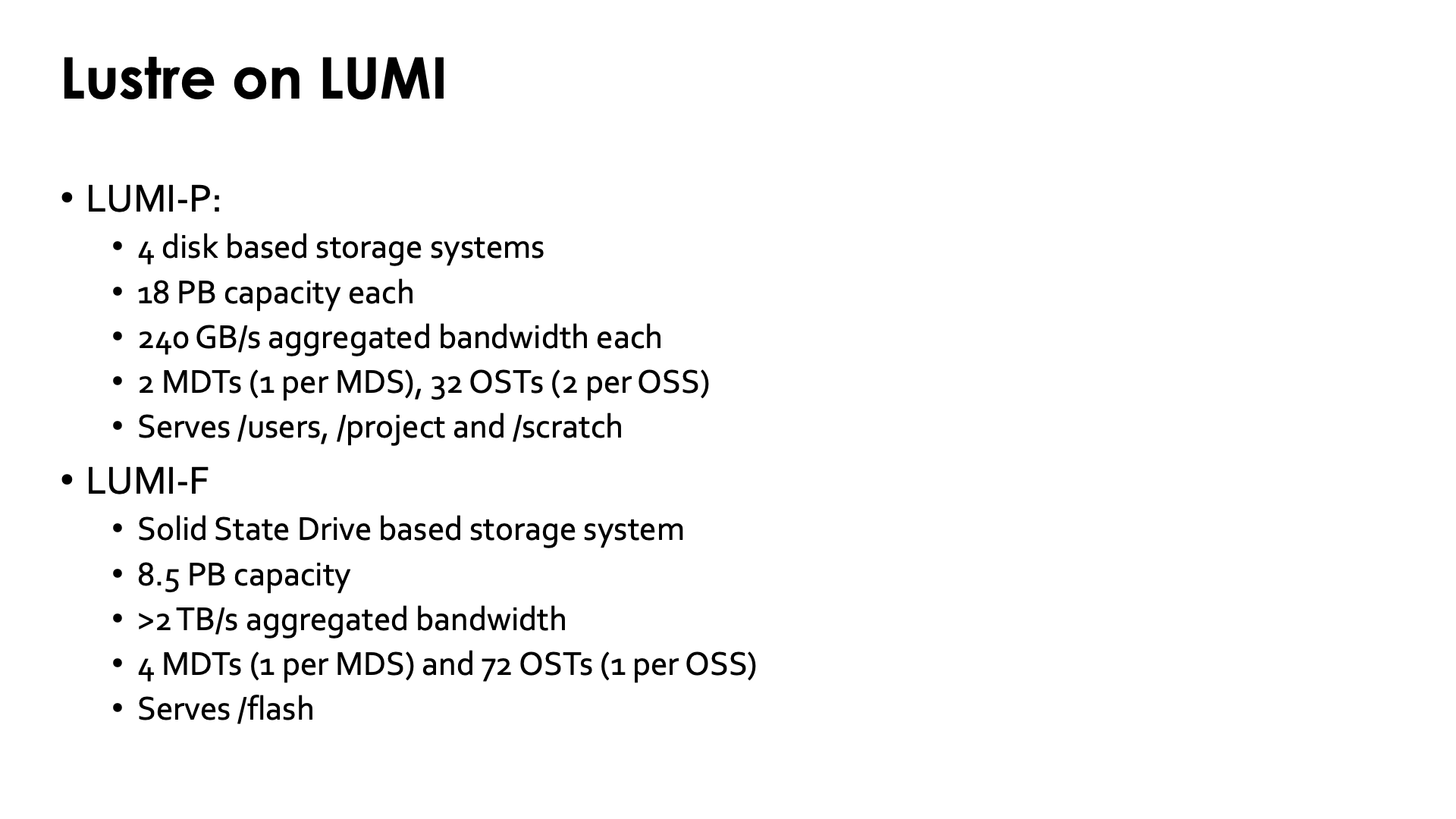
LUMI has 5 Lustre filesystems:

The file storage sometimes denoted as LUMI-P consists of 4 disk based Lustre filesystems, each with a capacity of roughly 18 PB and 240 GB/s aggregated bandwidth in the optimal case (which of course is shared by all users, no single user will ever observe that bandwidth unless they have the machine for themselves). Each of the 4 systems has 2 MDTs, one per MDS (but in a high availability setup), and 32 OSTs spread across 16 OSSes, so 2 OSTs per OSS. All 4 systems are used to serve the home directories, persistent project space and regular scratch space, but also, e.g., most of the software pre-installed on LUMI. Some of that pre-installed software is copied on all 4 systems to distribute the load.

The fifth Lustre filesystem of LUMI is also known as LUMI-F, where the "F" stands for flash as it is entirely based on SSDs. It currently has a capacity of approximately 8.5 PB and a total of over 2 TB/s aggregated bandwidth. The system has 4 MDTs spread across 4 MDSes, and 72 OSTs and 72 OSSes, os 1 OST per OSS (as a single OST already offers a lot more bandwidth and hence needs more server capacity than a hard disk based OST).

Links¶

The lfs command itself is documented through a manual page that can be accessed at the LUMI command line with man lfs. The various subcommands each come with their own man page, e.g., lfs-df, lfs-getstripe, lfs-setstripe and lfs-find.
Understanding Lustre Internals on the Lustre Wiki.
Lustre Basics and Lustre Best Practices in the knowledge base of the NASA supercomputers.
Introduction to DVS in an administration guide

Within the VSC, several of the Python trainings already pay attention to working efficiently with datasets in Python.
- Scientific Python. The current version of the slides contains a chapter on the use of HDF5. The GitHub repository with various examples, contains examples and a Jupyter notebook for HDF5 and examples and a Jupyter notebook for netCDF.
- Python for HPC. Not everything is mentioned on the web site, but the current version of the slides has at the end a chapter on I/O, mostly discussing using HDF5 in Python. See also these example files and Jupyter notebook on GitHub.
- Sometimes other data formats may be a better idea, e.g., in AI applications. With Python (and there exist such libraries for, e.g, C programmers), one can read directly from various archive file formats, e.g., gzip and tar files. See these examples from the VSC Python systems programming course
MPI courses will often also discuss MPI I/O which is a building block to implement proper I/O strategies in parallel applications, and is also used in the implementation of HDF5, netCDF and likely other libraries.
Jülich Supercomputer Centre (between Aachen and Köln) organises a lot of trainings. The annual training "Parallel I/O and Data Formats" is particularly relevant for this chapter of this tutorial.