Speed-up
Or: Using 100 processors should mean your job runs 100 times faster, right?
Speed-up and efficiency
Success in running on a parallel computer is often measured by looking at the speed-up, i.e., how much faster does a code run on X processors compared to on the smaller number \(Y\) processors, with \(Y\) typically one? So in a mathematical formula,
with \(T(X)\) the time on \(X\) processors and \(T(Y)\) the time on \(Y\) processors. Ideally \(Y = 1\) but in practice for big problems it is not feasible to measure \(T(1)\) because the problem doesn't fit in memory or simply takes too much time to run.
An alternative measure is the efficiency. When \(Y=1\), the efficiency is simply the speed-up divided by \(X\), i.e., this would be \(100%\) in the ideal case that using \(X\) processors also speeds up the computations with a factor of \(X\). The more general definition is
i.e., the total time spent by all \(Y\) processors (with \(Y\) ideally 1) divided by the total time spent by all \(X\) processors. Note that this is wall time and not some user time or user+system time reported by the operating system as one way one can lose efficiency is by simply not being able to use all resources continuously.
Amdahl's law and saturation
In the ideal case, running on \(X\) processors instead of \(1\) should make the application \(X\) times faster, but this is never the case. The graph below shows three scenarios.
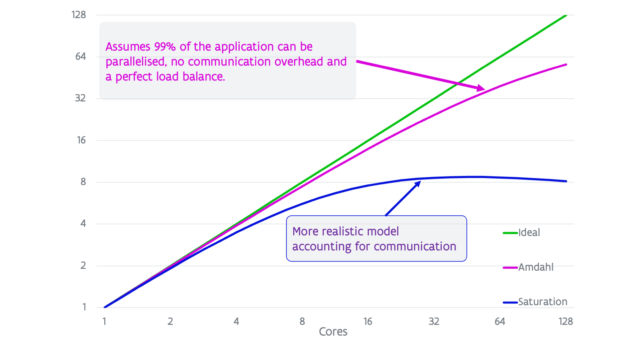
The top line (in green) shows the ideal speed-up. However, Amdahl noted already in the late '60s that using parallelism would have its limitations as every program will have some part that cannot be executed in parallel. Even if the parallel section could be executed on an infinite number of processors, the total run time would still be limited by that of the sequential part of the code. Assuming that \(99\%\) of the run time for a particular problem on one processor could be replaced by parallel code, then you could still never get a speed-up larger than 100 as there is that \(1\%\) of the runtime that cannot be eliminated. In fact, in later papers there was even a formula derived for this:
This curve is shown as the magenta line in the graph.
In reality the situation is even worse. Amdahl's law does not take communication overhead into account. In practice, the more processors are used the larger the relative communication overhead will become and this will lead to a saturation and even a lowering of the speed-up at some point as the number of cores is further increased. This is depicted in the lower line on the figure.
Amdahl's law already implies that whenever using parallel computing, one has to balance the cost of using more processors (as that cost will increase due to the efficiency loss) with the gain from getting an answer quicker. But this is even more pronounced in a more realistic situation.
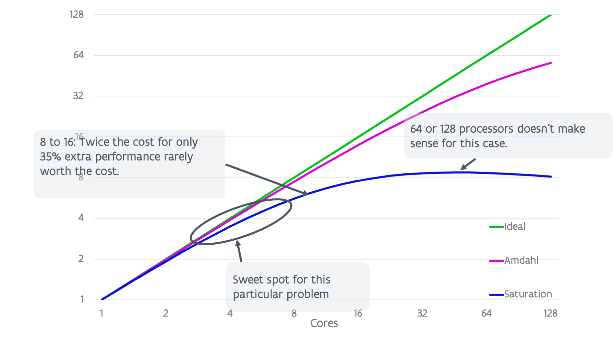
Looking at the blue curve (the lower one) in the above graph shows that it makes no sense to even use 64 or 128 cores for this particular problem as the speed-up is lower than for roughly 32 cores (and hence the execution time higher). However, going from 8 to 16 cores we also effectively gain only \(35\%\) performance so one can wonder if this is worth the cost. The sweet spot for this problem is probably somewhere between 4 and 8 cores.
What does this mean?
Using \(X\) times more processors will almost never speed up your application with a factor of \(X\) as there is always some overhead in using more cores. There are some rare cases where this is not the case though and where you may see what is called a superlinear speed-up. This is due to memory and cache effects. As you are using more cores, the problem per core becomes smaller and as a consequence more of it may fit into the caches, improving the performance of a core, or at a coarser level, if you're using more memory than is available per core in a machine when using a low core number, at some point the memory use per core will become small enough that each core only uses memory from its own NUMA domain.
There is also no rule like program A runs best on \(X\) processors. The optimal number of processors \(X\) does not only depend on the application that you're using. It also depends on the cluster: the characteristics of the CPU, the interconnect, ..., all have an influence on the number of cores that can be used with reasonable efficiency. In general, on supercomputers with a slower interconnect with less bandwidth or more latency, fewer cores can be used for any given problem, even if those cores are the same as on the computer with faster interconnect. But most importantly, the optimal number \(X\) of processors also depends on the problem being solved. As we will see further in this chapter, the bigger the problem, the higher the optimal number of cores. This is why a supercomputer support team cannot tell you: If you use VASP, then use that number of nodes.
The general rule is though that bigger problems give you a better speed-up and efficiency for a given number of cores, or let you use a larger number of processors for a given target efficiency.